03. Quick Start & In Depth Tutorial: Exploring BGCs in Cutibacterium
Please install lsaBGC as described on the Installation page and activate the conda environment before proceeding.
Also check out lsaBGC-Easy.py for an even quicker start!!!
As a quick start to getting acquainted with lsaBGC and the functionalities it offers, we recommend running the run_tests.sh bash script (with the lsaBGC conda environment activated). This script basically runs lsaBGC-Ready.py to perform BGC formatting, clustering into GCFs, and, optionally, expansion to identify homologous instances of GCFs in additional genomes at scale (could be in the 1000s!). Then it uses lsaBGC-AutoAnalyze.py to iteratively run the following for each GCF: visualization (using lsaBGC-See.py), evolutionary analysis + consensus report generation (see Google sheets screenshot below!;using lsaBGC-PopGene.py), and divergence to expected divergence calculations to infer horizontal gene transfer (using lsaBGC-Divergence.py). It can also automatically do GCF identification in metagenomic datasets if provided with metagenomic readsets + identify at base-resolution new SNVs never seen in assemblies (using lsaBGC-DiscoVary.py).
Here are the contents of the script:
#!/usr/bin/env bash

# Step 0: Decompress test_case.tar.gz and cd into it (remove previous de-compression attempt).
rm -rf test_case
tar -zxvf test_case.tar.gz
cd test_case/

# Step 1: create genome listing inputs for lsaBGC-Ready.py
listAllGenomesInDirectory.py -i Primary_Genomes/ > Primary_Genomes_Listing.txt
listAllGenomesInDirectory.py -i Additional_Genomes > Additional_Genomes_Listing.txt

# Step 2: create BGC prediction Genbank listing input for lsaBGC-Ready.py (using AntiSMASH)
listAllBGCGenbanksInDirectory.py -i Primary_Genome_AntiSMASH_Results/ -p antiSMASH \
	-f  > Primary_Genome_BGC_Genbanks_Listing.txt

# Step 3: run lsaBGC-Ready.py - with clustering of primary genome BGCs, expansion to
#         additional genomes, and phylogeny construction set to automatically run.
lsaBGC-Ready.py -i Primary_Genomes_Listing.txt -d Additional_Genomes_Listing.txt \
	-l Primary_Genome_BGC_Genbanks_Listing.txt -p antiSMASH -a \
	-c 8 -t -lc -le -o lsaBGC_Ready_Results/

# Step 4: run lsaBGC-AutoAnalyze.py - automatically run analytical programs for
#         visualization, evolutionary stats computation and single row per
#         homolog group/gene tables. Can also perform metagenomic analysis
#         if requested.
lsaBGC-AutoAnalyze.py -i lsaBGC_Ready_Results/Final_Results/Expanded_Sample_Annotation_Files.txt \
	-g lsaBGC_Ready_Results/Final_Results/Expanded_GCF_Listings/ \
	-m lsaBGC_Ready_Results/Final_Results/Expanded_Orthogroups.tsv \
	-s lsaBGC_Ready_Results/Final_Results/GToTree_output.tre \
	-w lsaBGC_Ready_Results/Final_Results/GToTree_Expected_Differences.txt \
	-u Genome_to_Species_Mapping.txt -c 8 -o lsaBGC_AutoAnalyze_Results/
In this tutorial we will use various lsaBGC tools and take a look at their output to showcase their application on a realistic scenario to explore the secondary metabolome of Cutibacterium. We will use the latest recommended workflows on Cutibacterium genomes featured in R202 of GTDB. Cutibacterium are highly abundant taxa on skin which we investigated in our recent manuscript introducing lsaBGC. Results achieved here will defer slightly from what we saw in the paper because we are using a different workflow featuring lsaBGC-Ready.py instead of lsaBGC-AutoProcess.py to simplify set up for lsaBGC analysis along with other adjustments to the initial workflow.
This tutorial assumes you are using a UNIX based operating system such as Linux or macOS. It can take a while to run with limited computational resources and we also suggest taking a look at the test cases which demonstrate running each of the 8 core lsaBGC programs with small datasets.
Tutorial Data:
Please download and uncompress the genomes and pre-computed antiSMASH results for 345 Cutibacterium featured in the GTDB release R202 currently hosted here on Google drive using the following command: tar -zxvf Cuti_Tutorial_Data.tar.gz.
Note, the uncompressed size of the data will be ~1.4GB.
Additionally, pre-computed antiSMASH results are only provided for 19 select representative genomes based on dRep dereplication analysis using standard parameters and fastANI for secondary clustering. AntiSMASH can be time-consuming to run and we typically use lsaBGC-AutoExpansion to quickly identify BGCs in additional genomes after defining GCFs based on BGCs from these primary genomes. lsaBGC-AutoExpansion has the added benefit of synchronizing boundaries between BGC instances belonging to the same GCF and being more sensitive at BGC detection when working with fragmented draft genome assemblies.
The sub-directories of the tutorial dataset are the following:
Cuti_Tutorial_Data/Primary_Genomes/              : primary genomes in FASTA format (to be used for *de novo* ortholog finding and defining GCFs)
Cuti_Tutorial_Data/Additional_Genomes/           : additional genomes in FASTA format (will be searched for homologous GCFs using lsaBGC-AutoExpansion)
Cuti_Tutorial_Data/Primary_AntiSMASH_Results/    : precomputed antiSMASH results for primary genomes
Species_Phylogeny.nwk                            : Species phylogeny constructed using [GToTree](https://github.com/AstrobioMike/GToTree)
Before we can use lsaBGC-Ready.py, we actually need to generate input files listing the individual files featured in the tutorial data:
- Create listings of the primary and additional genomes:
# lsaBGC conda env is active
listAllGenomesInDirectory.py -i Primary_Genomes/ > Primary_Genomes.txt
listAllGenomesInDirectory.py -i Additional_Genomes/ > Additional_Genomes.txt
- Create a listing of the antiSMASH results (only complete BGCs - not on contig edges!) for the primary genomes:
# lsaBGC conda env is active
# The "-f" argument specifies that only complete BGCs should be gathered (ie. to exclude those found on contig edges)
listAllBGCGenbanksInDirectory.py -i Primary_AntiSMASH_Results/ -p antiSMASH -f > Primary_AntiSMASH_BGC_Predictions.txt
Ok, great, we have all the files needed to get started with lsaBGC analysis! With the following command we will use the 3 listing files we just created to generate listing files and inputs needed for the core lsaBGC programs. We do not run lsaBGC-Ready.py with automatic clustering and expansion analysis similar to the small testing case as there are advantages to running these steps manually and to better showcase matters related to parameters users should consider. Optionally, lsaBGC-Ready.py can also take BiG-SCAPE results in place of performing clustering!
# lsaBGC conda env is active
lsaBGC-Ready.py -i Primary_Genomes.txt -l Primary_AntiSMASH_BGC_Predictions.txt \
                -d Additional_Genomes.txt --annotate --run_gtotree
                --cpus 8 --output_directory lsaBGC_Ready_Results/
Depending on what options you use the resulting files in the directory lsaBGC_Ready_Results/Final_Results/ will alter to show the most appropriate set of files to use for downstream lsaBGC analyses. This will generate the files needed for subsequent lsaBGC analysis. Note, primary genomes will also be appended to the additional genomes listing by default by lsaBGC-Ready.py to enable detecting BGCs which were not included because they were incomplete (near contig edges) via lsaBGC-Expansion.py later on.
Now that we have the major input files needed for lsaBGC analysis, we can perform clustering of BGCs into GCFs. To do this we usually want to do a preliminary run of lsaBGC-Cluster.py with the option --run_parameter_tests. This will generate a user-friendly PDF report with figures aimed to guide users to selecting the best parameters. Please see the lsaBGC-Cluster wiki page for more information. As mentioned above, lsaBGC-Cluster.py can optionally be run from within lsaBGC-Ready.py or BiG-SCAPE results could be provided to lsaBGC-Ready.py (overall the lsaBGC-Cluster and BiG-SCAPE algorithms are very similar with slight differences in graph clustering algorithm [affinity propagation vs. MCL] and syntenic similarity calculations).
# lsaBGC conda env is active
lsaBGC-Cluster.py -b lsaBGC_Ready_Results/Final_Results/Primary_AntiSMASH_BGCs.txt \
                  -m lsaBGC_Ready_Results/Final_Results/Orthogroups.tsv -o lsaBGC_Cluster_Results/ \
                  -r 0.7 --run_parameter_tests
From the report, we see that to minimize the number of singleton GCFs (GCFs with one BGC representative) yet to maximize the number of GCFs, we should set the Jaccard similarity cutoff for homolog groups shared between BGCs to be less than or equal to 50. We also see that the MCL Inflation does not matter much so we can leave it with the default value. Ok, so lets run the final clustering with this insight to get our gene cluster families (homologous groups of BGCs):
# lsaBGC conda env is active
lsaBGC-Cluster.py -b lsaBGC_Ready_Results/Final_Results/Primary_AntiSMASH_BGCs.txt \
                  -m lsaBGC_Ready_Results/Final_Results/Orthogroups.tsv \
                  -o lsaBGC_Cluster_Results_J00_R70/ -r 0.7 -j 0.0
We get 6 non-singleton and 3 singleton GCFs total. To get some basic stats one can view the file lsaBGC_Cluster_Results_J00_R70/GCF_Details_Expanded_Singletons.txt:
GCF id	number of BGCs	number of samples	samples with multiple BGCs in GCF	size of the SCC	mean number of OGs	stdev for number of OGs	min pairwise Jaccard similarity	max pairwise Jaccard similarity	number of core gene aggregates	annotations
GCF_1	8	8	0	11	17.875	0.9910312089651149	63.63636363636363	100.0	1	RRE-containing:8.0
GCF_2	6	6	0	9	10.666666666666666	0.5163977794943222	75.0	100.0	1	RiPP-like:6.0
GCF_3	5	5	0	34	36.8	1.7888543819998317	87.17948717948718	100.0	1	ladderane:5.0
GCF_4	2	2	0	44	47	0.0	88.0	88.0	1	NRPS-like:1.0; NRPS:1.0
GCF_5	2	2	0	6	8	0.0	60.0	60.0	1	RiPP-like:2.0
GCF_6	2	2	0	10	11.5	2.1213203435596424	76.92307692307693	76.92307692307693	1	RiPP-like:2.0
GCF_7	1	1	0	NA	10	0	0	0	0	RiPP-like:1.0
GCF_8	1	1	0	NA	15	0	0	0	0	RiPP-like:1.0
GCF_9	1	1	0	NA	22	0	0	0	0	thiopeptide:0.5; RRE-containing:0.5
So overall, because Cutibacterium do not have many BGCs, we see that we are able to get robust GCFs where a single GCF is found in at most one copy per genome. In more saturated taxa, such as Streptomyces, one can imagine GCFs where paralogous instances exist per genome.
The major resulting files are "GCF Listings" these are simple tab-delimited text files, one per GCF, which have a sample identifier as the first column and a path to a BGC prediction Genbank belonging to the GCF in the second column. This simple format allows users to modify them as they see fit. Should one of the BGCs actually be a separate GCF? - No problem just edit the GCF listing to remove that BGC instance! GCF Listings can be found in the subdirectory: lsaBGC_Cluster_Results_J00_R70/GCF_Listings/.
Running lsaBGC-AutoExpansion to Rapidly and Sensitively Identify Instances of GCFs Directly in Genomes
lsaBGC-AutoExpansion.py allows for rapid and sensitive GCF detection in genomes. lsaBGC-Expansion.py constructs profile HMMs for auxiliary homolog groups from GCFs and then uses a classical HMM to identify neighborhoods belonging to the GCF, similar to ClusterFinder. However, critically, it keeps track of whether BGC pieces are on contig/scaffold edges and has a conditional assessment to first determine if the GCF is present in a genome and second to report only fragments likely belonging to the GCF (even if they have no core biosynthetic domains because of assembly fragmentation). lsaBGC-AutoExpansion.py is a wrapper of lsaBGC-Expansion.py which simply runs the core program for each GCF and afterwards consolidates results by making sure that if overlapping BGCs are reported as belonging to multiple GCFs, the BGC region is assigned to its best match based on sequence similarity.
# lsaBGC conda env is active
lsaBGC-AutoExpansion.py -g lsaBGC_Cluster_Results_J00_R70/GCF_Listings/ -m lsaBGC_Ready_Results/Final_Results/Orthogroups.tsv \
                        -l lsaBGC_Ready_Results/Final_Results/Primary_Sample_Annotation_Files.txt \
                        -e lsaBGC_Ready_Results/Final_Results/Additional_Sample_Annotation_Files.txt \
                        -o lsaBGC_AutoExpansion_Results/ -q -c 8
After lsaBGC-AutoExpansion has run we will end up with the core set of files needed to run downstream lsaBGC analyses using:
lsaBGC_AutoExpansion_Results/Orthogroups.tsv :              Homolog group vs. sample presence/absence matrix with gene identifiers shown for presence.
lsaBGC_AutoExpansion_Results/Updated_GCF_Listings/ :        Updated GCF listings directory with BGCs detected in additional genomes also included for each GCF listing text file.
lsaBGC_AutoExpansion_Results/Sample_Annotation_Files.txt :  Sample annotation file paths for both primary and additional genomes.
Note, gene identifiers for primary genomes will have locus tags of length 3 (e.g. ABC_000001) whereas additional genomes will have locus tags of length 4 (e.g. ABCD_000001). lsaBGC uses this information for certain tasks (including in lsaBGC-Expansion.py), primarily because paralogs of GCF associated homolog groups are only searched in a genome-wide fashion for primary genomes and statistics of homolog group specificity to be part of biosynthetic machinery is determined based on this search.
To showcase the following lsaBGC programs, we will focus in on just one GCF, GCF-9, which also corresponds to the thiopeptide cutimycin recently described by Claesen et al. 2020. These following lsaBGC cpus allow users to investigate individual GCFs at scale to uncover interesting patterns and prioritize GCFs to further pursue for discovery of commercialisable natural products.
Note, however, typically, we run lsaBGC-AutoAnalyze.py which is a workflow to run the core programs lsaBGC-See.py (for visualization), lsaBGC-PopGene.py (compute evolutionary stats + generate convenient report overview of each GCF), and lsaBGC-Divergence.py (computes Beta-RD, an indicator of how diverged in sequence GCF genes are relative to expected divergences based on ANI/AAI or, now, with the incorporation of GToTree, the divergence exhibited by single-copy core proteins. lsaBGC-AutoAnalyze.py will also generate a consolidated table of each GCF's lsaBGC-PopGene.py report which can be used to get a quick sense of the secondary metabolome of the taxa and explore functional (through annotation) + evolutionary statistics to identify key GCFs of interest! It will also generate some big-picture overview figures. For more information on lsaBGC-AutoAnalyze, check out its Wiki page and its usage in the Quick Start part of this page (up above!).
Generating a Summarized Report for a GCF with Functional, Syntenic and Evolutionary Information Easily Summarized
Perhaps the most useful feature of lsaBGC for most will be its ability to generate consolidated reports of homolog groups found in different instances of a GCF (each homolog group is a row). This report is by default ordered according to the consensus order of homolog groups across GCF instances (consensus direction also reported). For each homolog group, functional information, evolutionary stats, and conservation across samples are reported and gives a nice view for users to get a quick glance at the GCF at large! Information on all 20+ columns in these reports can be found on the lsaBGC-PopGene wiki page.
One of the evolutionary statistics lsaBGC-PopGene.py reports per homolog group is called Beta-RD which is just the median of nucleotide or protein similarity of homologs divided by the genome-wide ANI or AAI of the corresponding genomes. Beta-RD is 1 if sequence divergence of the homolog group is as expected based on genome-wide divergence. If it is greater than 1 then sequence divergence is less than expected and might indicate conservation or horizontal gene transfer. To calculate genome-wide pairwise differences we previously used the script computeGenomeWideDistances.py (but no longer recommend due to more involved installations), so instead we recommend simply specifying --run_gtotree option which will automatically create a species phylogeny and also use the basis alignment of single copy core genes to estimate expected divergences of pairs of samples/genomes. Users can however perform an ANI or AAI analysis using fastANI or CompareM as we did for Salamzade et al. 2022 for more accurate estimations. This file is simply a three column tab-delimited text file listing the first sample (1st column), second sample (2nd column), and the ANI/AAI/Expected-Divergence on a 0.0 to 1.0 scale (3rd column).
We can next run lsaBGC-PopGene.py, because I won't be diving into evolutionary stats much in this tutorial, we won't provide a dereplicated sample set with the -k argument, but this is generally recommended as such statistics (including Tajima's D, dN/dS and population genetic stats) can be influenced by representation bias. Again this sample set can be selected through dRep or the method provided in computeGenomeWideDistances.py.
# lsaBGC conda env is active
lsaBGC-PopGene.py -g lsaBGC_AutoExpansion_Results/Updated_GCF_Listings/GCF_9.txt -m  lsaBGC_AutoExpansion_Results/Orthogroups.expanded.tsv \
                  -i GCF_9 -o GCF_9_PopGene/ -c 4 -w lsaBGC_Ready_Results/Final_Results/GToTree_Expected_Differences.txt
Here is a screenshot of the report produced for the GCF, GCF_9_PopGene/Homolog_Group_Information.txt, after I pasted it into Google sheets and highlighted some cells:
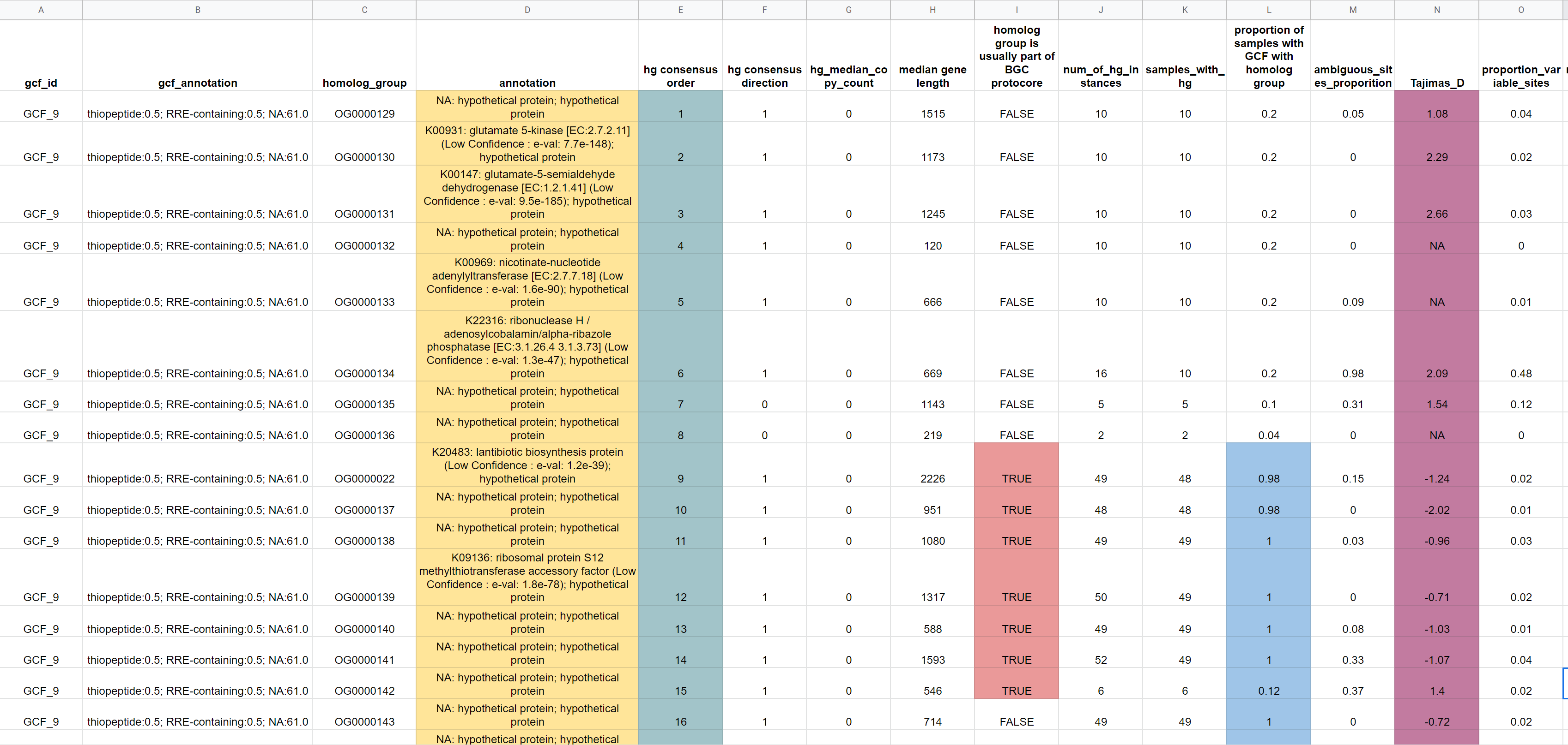
Starting from the left, you can see each row corresponds to a different homolog group. The annotation based on KOfam is shown (highlighted in yellow). Next, in teal we have the consensus homolog group order, we can see the rows are already ordered accordingly. In red, we have cells indicating that the corresponding homolog groups are often (>50% of primary BGC instances) found in protocore regions as defined by antiSMASH predictions. The proportion of samples with GCF-9 which have the homolog group is then shown in blue. We see that around the protocore homolog groups conservation is high. Finally, we have the Tajima's D statistic which can be used to determine whether homolog groups are under selective pressures and how much sequence variability there is (but again genome representation and dereplication should be considered).
Users can additionally find summarized visualizations of homolog group codon-alignments in the lsaBGC-PopGene.py results directory under Codon_MSA_Plots/.
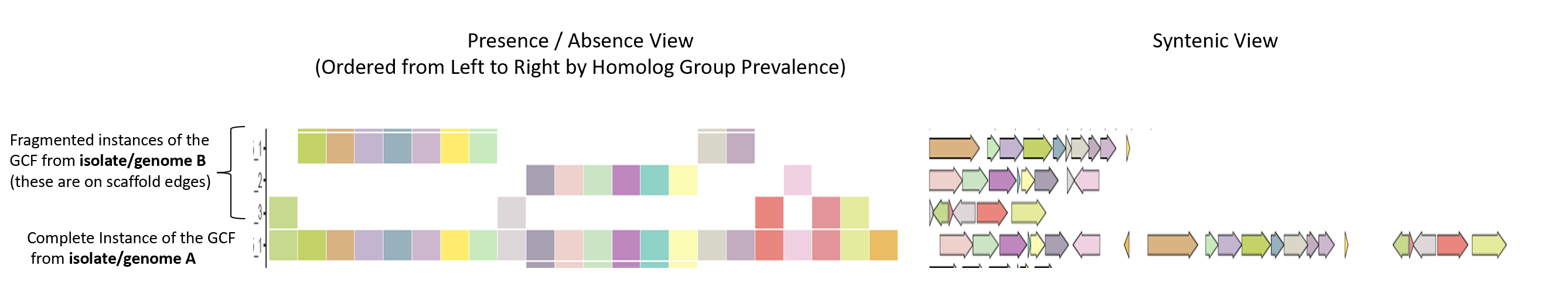
lsaBGC-See.py lets users visualize GCF micro-synteny schematics across a species phylogeny (compared to CORASON which builds gene-specific phylogenies). A key feature of lsaBGC-See.py is its consideration of draft genomes containing split-up / fragmented GCFs. It splits up leaves corresponding to such genomes where there are two or more genomic regions corresponding to the same GCF and visualizes them side-by-side to allow users to jig-saw together a complete picture of the GCF in the genome:
# lsaBGC conda env is active
lsaBGC-See.py -g lsaBGC_AutoExpansion_Results/Updated_GCF_Listings/GCF_9.txt -m lsaBGC_AutoExpansion_Results/Orthogroups.expanded.tsv  \
              -o GCF_9_See/ -i GCF_9 -s lsaBGC_Ready_Results/Final_Results/GToTree_output.tre -c 4
Here is the default view produced with some R graphics, iTol tracks are also created along with the altered variant of the phylogeny (to expand leaves when multiple BGCs found per genome):
Additional programs featured in lsaBGC but not highlighted in this tutorial include:
- Using
lsaBGC-Discovary.pyto perform base-resolution mining in metagenomic datasets - Using
lsaBGC-Divergence.pyandcompareBGCtoGenomeCodonUsage.pyto infer instances of BGC sequence similarity or codon usage between two genomes not matching expectations based on genome-wide comparisons. These were used in our study to determine instances of horizontal gene cluster transfer. - Systematic refinement of GCF boundaries by user defined boundary homolog groups using
lsaBGC-Refiner.py
Testing data with expected outputs can additionally be found at this Git repo. Together with specific commands and input data, expected results and computation runtimes are also provided.