Response

Dear Editor and Reviewers:

Please find attached our revised manuscript for PVLDB Volume 18 (VLDB'25), originally submitted as paper #1354. We received the decision with "Revision", and we sincerely thank the editor and reviewers for their constructive feedback, which has significantly strengthened our work. Below is a summary of our key revisions:

• Formal Complexity Analysis: Add a formal complexity analysis of eXpath's path-based rule mining algorithm and quantify the complexity of the path aggregation method via empirical experiments (Sections 4.1-4.2, Figure 1).

• User-Centric Evaluation: Conduct an in-lab user study on the visualization prototype of eXpath against other methods. Collect, analyze, and report qualitative feedback on the explanation's effectiveness, rationality, and clarity. Also, expand discussions on user personas (domain experts and data scientists) (Sections 3, 5.3, Figure 2).

• Justification of Assumptions and Design Choices: Justify the alignment of graph patterns (CP/PT rules) with embedding-based models and explain why critical facts are always adjacent to the head/tail of the predicted link (Sections 4.1, 4.3, Table 1).

• Extension of Quantitative Experiments: Add a comparison with KE-X (Section 5.2), clarify evaluation metrics (e.g., $\delta$MRR, batch adversarial attacks, fusion methods) in Section 5.1, and restructure Sections 5.3 (Fact Position Preferences) and 5.4 (Ablation Study on Rule Components) to highlight key findings more prominently.

• Expansion of Related Work: Enhance the discussion in Section 2.2 by introducing a new dichotomy for adversarial attack methods and comparing how Kelpie (single-hop links), KGEAttack (limited 2-hop rules), and eXpath (multi-hop paths) handle the example in Figure 1.

• Visualization and Case Study Improvements: Present unified case examples across figures (Fig. 1, 2) for consistency, revise the layout of the pipeline visualization (Figure 3) to improve its clarity, and update the case study to include a comparison with Criage and DP.

All changes are highlighted in dark red in the revised manuscript, which is appended at the end of this document (pp.28-40). Elaborate responses to the feedback from each reviewer are provided following this letter (pp.3-27). We look forward to hearing from you about any further comments and suggestions. Thank you for considering the paper.

Yours Sincerely,

Ye Sun, Lei Shi, Yongxin Tong

---

Reviews and our reply

PVLDB Editor

Review: While the individual reviewers have specified individual revision requests in their reviews, we provide the following summary of revision requests:

M1: Justification of underlying assumptions and design choices
M2: Formal complexity analysis or discussion of computational complexity
M3: Expansion of related work, e.g., with clarifying examples, to make the arguments more clear.
M4: Clarifying the unclarities that the reviewers found in the experiments, the methodology applied for the experiments, and add a comparison against KE-X [41].

Reply: Thank you for your summary of the revision requests. We have addressed all the issues raised by the individual reviewers, and the corresponding changes have been incorporated into the revised manuscript. Below, we provide a brief summary of how we have addressed these requests.

M1: Justification of Underlying Assumptions and Design Choices
The alignment between graph patterns (CP/PT rules) and embedding-based models is grounded in their mathematical design. CP rules (e.g., $r \leftarrow r_1, r_2$) in TransE utilize additive operations ($\mathbf{h} + \mathbf{r}_1 + \mathbf{r}_2 \approx \mathbf{t}$) to reflect path composition, while ComplEx employs matrix multiplications ($\mathbf{h} \cdot \mathbf{R}_1 \cdot \mathbf{R}_2 \approx \mathbf{t}$) to capture hierarchical dependencies. Similarly, PT rules (e.g., $\texttt{country}(X, \text{Japan}) \leftarrow \texttt{language}(X, \text{Japanese})$) are based on geometric co-occurrence. These operations ensure that models implicitly learn relational chains encoded in CP rules and co-occurrence in PT rules.

The prioritization of head/tail-adjacent critical facts is guided by two principles: (1) Embedding sensitivity ensures direct facts (e.g., $\langle h, r_1, A \rangle$) primarily influence $h$/$t$ embeddings, while intermediate facts have weaker effects. (2) Empirical analysis on FB15k-237 demonstrates that head/tail-adjacent facts exhibit much higher mean contribution ($p_h = 0.0217$, $p_t = 0.0037$) than non-adjacent facts ($p_m = 0.0005$), with 99.8% of non-adjacent facts contributing negligibly ($p_m < 0.01$). This means that adjacent facts are more likely to be shared across multiple paths within a rule, making them more critical for explaining the prediction.

M2: Formal Complexity Analysis
The computational complexity of eXpath's path-based rule mining is rigorously analyzed. The key components include: Here we analyze the complexity of Algorithm 1, which consists of the following components: (1) the bidirectional BFS search for generating candidate paths, with a complexity of $O(d^{\frac{L}{2}})$, where $d = \frac{2M}{N}$ is the average node degree, $L$ is the maximum path length, and $N$, $M$, and $R$ denote the number of nodes, edges, and relations respectively.; (2) path aggregation, which merges paths by relation sequences and results in $|\mathcal{P}_{r}| = O(\min{d^{\frac{L}{2}}, R^L})$; (3) local optimization, which trains on a subgraph of size $O(d)$ with a complexity of $O(d T)$, where $T$ is the model-specific training cost (e.g., $O(D)$ for TransE and $O(D^2)$ for RESCAL, where $D$ represents the dimension of embeddings); and (4) rule evaluation, which scans training facts with a complexity of $O(M L)$ for $L$-hop paths. Thus, the overall complexity is $O(\min{R^L, d^{\frac{L}{2}}} \cdot (ML + dT))$, dominated by $O(M)$, as $L$, $d$, $R$ and $T$ are limited by dataset characteristics or predefined bounds. This linear scalability facilitates the effective application of large-scale KGLP tasks' explanations.

M3: Expansion of Related Work
Section 2.2's discussion has been enhanced by explicitly contrasting how different methods handle the example in Figure 1. For instance, Kelpie prioritizes single-hop links (e.g., material properties) as explanations, while KGEAttack, despite considering 2-hop rules, struggles to identify longer paths like the 3-hop co-occurrence path in Figure 1. These enhancements clarify the distinct strengths of eXpath in offering path-based explanations aligned with expert preferences for semantic-rich, multi-hop reasoning, making the arguments more transparent and concrete.

M4: Experiment Clarifications and KE-X Comparison
We have incorporated KE-X into our experiments (Section 5.2), clarified evaluation metrics (e.g., $\delta$MRR, batch adversarial attacks, fusion methods), and restructured Section 5.3 (Fact Position Preferences), and Section 5.4 (Ablation Study on Rule Components), to highlight key findings more prominently. These studies indicate that restricting explanations to head-related facts leads to better performance, CP rules form the foundation of eXpath's reasoning, and PT rules enhance explanation diversity.

Reviewer 1

Review 1: User of Explanations.

The paper discusses semantic explainability but does not define who benefits from these explanations. Are they for data scientists, domain experts, or general users? Adding a discussion on user personas and their expectations would strengthen the argument for semantic explainability. The case study would be more impactful if it included a discussion of who was analyzing the explanations and what their needs were. If possible, incorporate a small-scale user study or qualitative analysis. This would improve the credibility of the claim that the approach enhances human interpretability.

Reply: "Thank you for your valuable feedback on clarifying user personas and enhancing the case study with user-centric analysis. We have incorporated your suggestions into the paper. Specifically, in Section 3.3, we have included a new paragraph that delineates the primary user groups, namely domain experts and data scientists, along with their respective needs. We highlight how CP/PT rules cater to the structured reasoning requirements of domain experts, such as causal paths in materials science, and fulfill data scientists' demand for model transparency. Furthermore, we have enriched the FB15k case study (Section 5.3) by explicitly identifying the evaluators as data scientists and domain experts, along with elucidating their criteria for validating explanations. For instance, domain experts affirmed that rules like $\texttt{country(X, Japan) ← language(X, Japanese)}$ are in line with linguistic-geographic common sense, while data scientists pointed out that such rules showcase the ability of embedding models to capture inter-domain relationships."

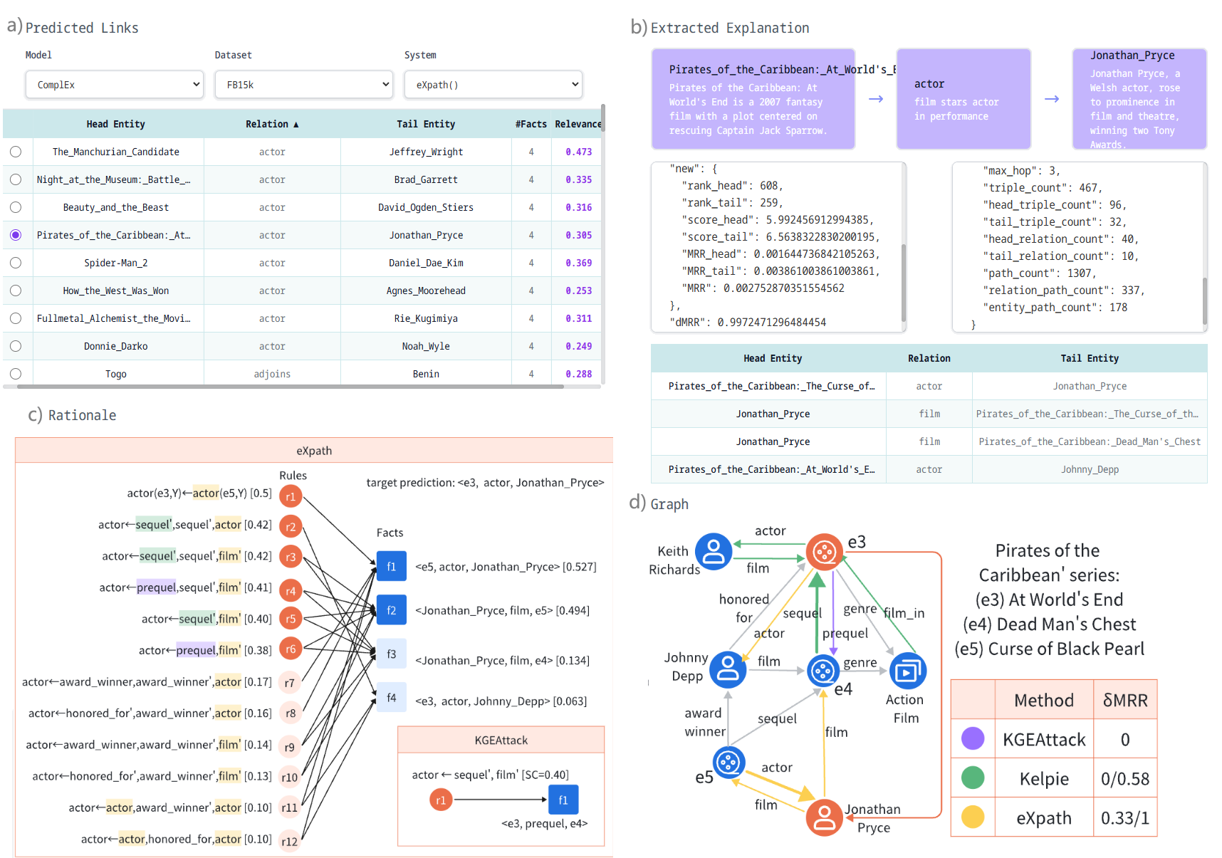
Figure 1: Visualization prototype consists of four components for interaction and analysis: (a) Predicted Links for selecting target predictions, (b) Extracted Explanation for displaying explanations extracted by different methods, (c) supporting rationales for showing how the facts are selected and (d) Graph for visualizing local KG structure.

To assess the effectiveness, rationality, and clarity of explanations produced by eXpath, KGEAttack, and Kelpie, we carried out a small-scale in-lab user study involving five researchers specializing in graph-related research. Three prototype diagrams were developed to serve as case study examples. Each diagram featured the following components: (a) the predicted link, (b) explanations from eXpath, KGEAttack, and Kelpie accompanied by their $\delta MRR$ performance metrics, (c) supporting rationales demonstrating how rules (e.g., eXpath's $\texttt{actor(e3,Y) ← actor(e5,Y) [0.5]}$) underpin the selection of facts (e.g., $\langle e5, \text{actor}, \text{Jonathan Pryce}\rangle$ [0.527]"), and (d) a graphical representation of entities and relationships. Participants examined these prototypes and shared qualitative feedback through open-ended questionnaires.

For "effectiveness," eXpath demonstrated superior performance compared to KGEAttack and Kelpie. The majority of participants (4 out of 5) found eXpath's explanations more convincing due to the incorporation of diverse facts rather than focusing solely on head-related facts. One participant highlighted that "eXpath's utilization of analogy and co-occurrence rules resonates with how I would verify actor-film connections, unlike the limited scope of KGEAttack." In terms of "rationality," both eXpath and KGEAttack received acclaim for anchoring explanations in rules (e.g., $\texttt{actor ← sequel, sequel, actor [0.42]}$), while Kelpie's lack of rationale caused confusion. A participant commented, "The absence of path-based rationale in Kelpie's explanation gives the impression of arbitrariness." Regarding "clarity," some individuals initially found eXpath's multi-step rule-to-fact selection overwhelming ("Too many rules clutter the logic"), but this issue was alleviated by the graph visualization of rationale (see Figure 2(c)), which facilitated the mapping of rules to facts. While KGEAttack's simpler rules were easier to comprehend, they were deemed less informative.

The study underscores eXpath's strength in balancing semantic depth and transparency. Advanced visualization tools, as previewed in the prototypes, will further bridge complex rules and user understanding.

Review 2: Emphasize Key Insights from the Ablation Study.

Important details from the ablation study are somewhat buried. Consider restructuring the results section to highlight key findings more prominently. The current conclusion section is really a summary. Have a conclusion section that truly provides conclusions and this is where you can share the insights.

Reply: Thank you for your valuable feedback. We have revised the ablation study section to highlight key findings more prominently and connect them to broader implications for knowledge graph (KG) reasoning. In summary, we present the following insights and their significance:

• Distinct Roles of CP and PT Rules: The ablation study reveals that CP (Compositional Path) rules are the backbone of eXpath's reasoning, capturing multi-hop relational patterns essential for semantic understanding.
• Dataset-Specific Rule Dominance: The impact of CP and PT rules varies across datasets, reflecting their adaptability to different relational structures.
• Ineffectiveness of Other Rule Types: Experiments with additional rule types—such as unary rules with dangling atoms—show negligible impact, validating our focus on CP and PT rules.

The synergy between CP and PT rules bridges the gap between symbolic (rule-based) and subsymbolic (embedding-based) reasoning, providing semantically grounded explanations that align with human understanding. These insights have been integrated into Section 5.4 and the conclusion of the revised manuscript.

Review 3: Future Work: Toward a User Study.

While this paper focuses on the technical aspects, a natural next step would be a user study assessing whether the explanations improve understanding and decision-making Given that explainability is highly user-dependent, it would be very interesting to study whether the generated explanations are too high-level or too technical for different audiences.

Reply: We have proposed a forthcoming user study in the Conclusion (Section 6) to assess the interpretability of eXpath's explanations. In this endeavor, we have developed a prototype for visualization to exhibit paths, rules, and supporting facts related to specific predictions. This design is intended to improve the accessibility and comprehension of eXpath's explanations for both knowledgeable KG professionals and non-expert users. The specifics of this interface and its operations have been incorporated into Section 6 of the revised manuscript.

Furthermore, we acknowledge the necessity of a thorough user study to validate the efficacy of our approach. In the future, our intention is to refine the visualization further and carry out a specialized user study involving experts in the field and data analysts. This study will assess the clarity, relevance, and actionability of eXpath's explanations using criteria such as clarity (rated on a 1-5 Likert scale) and actionability (Yes/No). We believe this forthcoming research will offer valuable insights into the human interpretability of path-based explanations. These plans have been outlined in Section 6 of the revised manuscript.

Reviewer 2

Review 1: There is an underlying assumption that the considered graph patterns can be detected by embedding-based LP models, which needs further justification.

Reply: Thank you for your insightful comment on the capability of embedding-based LP models to capture graph patterns. This assumption is pivotal for the validity of eXpath. Our framework introduces CP and PT rules as explanations for the predictions made by embedding-based LP models. It is essential that these models adhere to the rationales we propose. Failure to learn or reflect the patterns defined by CP and PT rules would result in our explanations misrepresenting the actual basis for their predictions.

Embedding-based LP models are inherently designed to capture structural patterns in knowledge graphs through their mathematical operations in embedding space, aligning naturally with graph pattern definitions. For CP rules, which encode multi-hop relational chains like $r(A_0, A_n) \leftarrow r_1(A_0, A_1) \land \dots \land r_n(A_{n-1}, A_n)$, the compositional nature of embedding models allows them to detect such patterns. In TransE, the sequential translation mechanism $\mathbf{A_0} + \mathbf{r_1} + \dots + \mathbf{r_n} \approx \mathbf{A_n}$ directly mirrors the chaining logic of CP rules. If an alternative path exists between the head and tail entities, the embedding model learns to align the vector sum of the relation path with the target relation. For instance, in the path $\texttt{$e_3$} \xrightarrow{\texttt{sequel'}} \texttt{$e_4$} \xrightarrow{\texttt{film'}} \texttt{Jonathan Pryce}$, the model ensures that $\mathbf{r}{\texttt{sequel'}} + \mathbf{r}{\texttt{film'}} \approx \mathbf{r}_{\texttt{actor}}$, reflecting the CP rule's semantic intent. ComplEx extends this through matrix multiplication ($\mathbf{A_n} \approx \mathbf{A_0} \cdot \mathbf{R_1} \cdot \dots \cdot \mathbf{R_n}$). When the learned relation path closely matches the target relation, the CP rule is effectively captured by the model.

Similarly, PT rules, which model co-occurrence relationships such as $r(X, c) \leftarrow r_0(X, c')$, are also well-aligned with embedding-based models. In TransE, the fixed embeddings of anchor entities $c$ and $c'$ enforce geometric consistency. For example, in the rule $\texttt{country(X, Japan)} \leftarrow \texttt{language(X, Japanese)}$, the embedding of "Japan" ($\mathbf{c}$) and "Japanese" ($\mathbf{c'}$) are constrained such that $\mathbf{c} \approx \mathbf{c'} + \mathbf{r}_0$, where $\mathbf{r}_0$ represents the relationship between language and country. This ensures that any entity $X$ linked to "Japanese" via $\texttt{language}$ will maintain a predictable offset to "Japan" in the embedding space, aligning with the PT rule's semantic intent. In ComplEx, this co-occurrence is modeled through bilinear interactions ($\mathbf{c} \approx \mathbf{c'} \odot \mathbf{R}_0$), where the relation matrix $\mathbf{R}_0$ preserves the logical mapping between entities.

While embedding-based LP models excel at capturing CP and PT rules, they may struggle with more complex graph patterns. Higher-order logical rules, such as recursive dependencies (e.g., $\texttt{ancestor}(X, Y) \leftarrow \texttt{parent}(X, Z) \land \texttt{ancestor}(Z, Y)$) or rules with variable predicates (e.g., $\texttt{profession}(X, Y) \leftarrow \texttt{R}(X, Z) \land \texttt{profession}(Z, Y)$), require iterative or nonlinear operations that TransE's linear translations and ComplEx's bilinear products cannot inherently capture. This limitation highlights the importance of selecting rules that are within the expressive capacity of embedding models. CP and PT rules represent a reasonable and well-defined scope of patterns that embedding-based LP models can effectively learn and reflect.

Review 2: The mimic-based scoring relies on access to the model's plausibility function, making it less of a black-box approach. Please clarify and discuss implications.

Reply: Thank you for your insightful feedback on the black-box assumption in our mimic-based scoring approach. This is an excellent point about eXpath's mimic strategy not being purely black-box. Indeed, we acknowledge that the technique involves adjustments to entity embeddings during the post-training process, which distinguishes it from black-box methods. To provide greater precision, we propose framing the distinction not as a "white-box" versus "black-box" dichotomy but rather as a spectrum between model-dependent methods (requiring detailed architectural knowledge) and model-agnostic methods (operating across architectures with minimal adaptation).

The mimic-based scoring in eXpath is built upon Kelpie's post-training framework, which interacts with the model's embedding mechanism. This interaction includes initializing and adding mimic entities to the embedding matrix while preserving the original embeddings. These steps do require access to internal embeddings and scoring functions, technically aligning eXpath with white-box execution.

However, unlike traditional white-box approaches (e.g., Criage or Data Poisoning), which rely on gradients, loss functions, or architecture-specific manipulations, eXpath is designed to be model-agnostic. It does not depend on theoretical insights into the model's internal mechanics, such as gradient computations or architectural constraints. Instead, adapting eXpath to new embedding models (e.g., TransE, ComplEx, or RotatE) only requires minimal interfaces—primarily the ability to initialize embeddings and compute plausibility scores. This stands in contrast to gradient-based methods, which often require extensive theoretical derivations tailored to each architecture.

In light of your feedback, we now explicitly characterize eXpath as a model-agnostic method with white-box execution, distinguishing it from both gradient-driven white-box approaches (model-dependent) and purely black-box techniques. This hybridity allows it to leverage model signals (via embedding interactions) while maintaining practical flexibility (via low adaptation overhead). We have revised Section 2.2 of the manuscript to reflect this refined classification and are grateful for your input, which has significantly strengthened our discussion.

Review 3: A complexity analysis of the method would be valuable.

Algorithm 1: Path-based Rule Mining Algorithm

Input: Prediction f = ⟨h,r,t⟩, Facts from Training Set G_train
Output: Candidate Rule Set for Prediction Φ
1: Φ ← ∅
2: // Step 1: CP Rule Extraction
3: P ← BFSSearch(h, t) // O(d^{L/2}), bidirectional BFS with max depth L
4: P_r ← Aggregation(P) // O(P)=O(d^{L/2}), group paths by relation sequences
5: for each p in P_r do // O(P_r)=O(min{d^{L/2},R^L})
6: h, h', t, t' ← localOptimization(f, p, G_train) // O(dT)
7: Rel_h ← 1 - f_r(h', t)/f_r(h, t), Rel_t ← 1 - f_r(h, t')/f_r(h, t) // O(1)
8: if Rel_h > 0 and Rel_t > 0 then
9: (HC, SC, supp) ← RuleEvaluation(r←p, G_train) // O(ML)
10: if SC ≥ minSC and HC ≥ minHC then
11: Φ ← Φ ∪ {ϕ_CP: r ← p [SC × supp/(supp+minSupp)]} // O(1)
12: end if
13: end if
14: end for
15: // Step 2: PT Rule Extraction (Take Head PT Rule as Example)
16: F_train^h ← SearchFacts(h, G_train) // O(d), retrieve facts for head entity
17: for each ⟨h,r_0,t_0⟩ in F_train^h do // O(d)
18: (HC, SC, supp) ← RuleEvaluation(r(X,t)←r_0(X,t_0), G) // O(M)
19: if SC ≥ minSC and HC ≥ minHC then
20: Φ ← Φ ∪ {ϕ_PT: r(X,t) ← r_0(X,t_0) [SC × supp/(supp+minSupp)]} // O(1)
21: end if
22: end for
23: return Φ

Reply: Thank you for this suggestion. We agree that complexity analysis is crucial, which is why we have thoroughly analyzed the key component of our pipeline, namely the Path-based Rule Mining Algorithm. We have annotated the complexity of each step in the algorithm and provided a detailed analysis in the following paragraphs. We also add a paragraph for complexity analysis in Section 4.2.

First, let us define some key symbols: $N$ represents the number of nodes, $M$ the number of edges, $R$ the number of relations, $L$ the maximum path length ($L\leq 3$ in our case), and $d$ the average node degree, which can be expressed as $d = \frac{2M}{N}$. For a specific prediction, let $P = |\mathcal{P}|$ denote the number of paths related to the prediction, and $P_r = |\mathcal{P}_r|$ the number of relation paths. The BFS Search process begins with generating candidate paths $\mathcal{P}$ through bidirectional BFS, which has a time complexity of $O(d^{\frac{L}{2}})$.

Path Aggregation merges paths of the same relation type based on whether their relation sequences are identical. Since the number of relation types is limited (to $R$), the number of relation paths after aggregation theoretically satisfies $P_r \leq \min{R^L, P}$, i.e., $P_r = O(\min{R^L, d^{\frac{L}{2}}})$. However, in practice, because paths between two entities in a knowledge graph are always semantically constrained, $P_r$ is significantly smaller than $P$ after aggregation, especially for large datasets. Empirical studies across datasets like FB15k and WN18 show that $\frac{P_r}{P} = 0.03$ and $\frac{P_r}{P} = 0.17$, respectively. We hypothesize a power-law relationship between $P_r$ and $P$, i.e., $P_r \leq A \cdot P^{\frac{1}{k}}$, which in logarithmic space translates to $\log P_r \leq a + \frac{1}{k} \cdot \log P$.

We experimentally validate this on our datasets, as shown in Figure 1. By grid-searching for $k$ to ensure that at least 90% of the data points in each dataset satisfy $\log P_r \leq a + \frac{1}{k} \cdot \log P$, and ensuring that the $a$ values across the four datasets are within the same order of magnitude, we find $k = 2$. This experimentally suggests $P_r = O(P^{\frac{1}{2}})$. In complexity analysis, we still use the worst-case bound, i.e., $P_r = O(\min{R^L, d^{\frac{L}{2}}})$.

Figure 2: The experimental fitting between relation path count (Pr) and regular path count (P). The X/Y-axis are in the log scale. The dashed lines represent the fitted bounds of the form $log(Pr) \leq a +\frac{1}{k} \cdot \log(P)$, ensuring 90% of the data points satisfy the inequality.

Local optimization introduces two mimic entities, $h'$ and $t'$, and trains on a local subgraph after excluding related triples. The size of this subgraph, in terms of the number of triples, is $O(d)$. Assuming the training complexity on a unit dataset size is $O(T)$, the total complexity for this step is $O(d T)$. Note that $T$ is a model-specific parameter related to the number of training epochs and the complexity of a single training iteration. For example, TransE has a complexity of $O(D)$ (involving vector addition and subtraction, where $D$ is the embedding dimension), while RESCAL involves vector-matrix multiplications ($D \times D$ relation matrix) and has a complexity of $O(D^2)$.

Rule evaluation computes metrics like head coverage ($HC$) and confidence ($SC$) by scanning training facts. While this involves matrix multiplication, specifically multiplying adjacency matrices $S(r_1, r_2, r_3)$ of size $N \times N$, the relation matrices in knowledge graphs are typically highly sparse (each entity connects to only a few relations). Thus, instead of explicitly computing the entire matrix, we only perform combination matching on existing relation triples (e.g., $\left\langle e_i, r_1, e_j\right\rangle, \left\langle e_j, r_2, e_k\right\rangle$). Each match has a complexity of $O(M)$, and for an $L$-hop path, $L-1$ matches are required. Therefore, the overall complexity of rule evaluation is $O(M L)$.

The complexity analysis for PT Rule Extraction is similar. The SearchFacts step retrieves all triples connected to $h$, which is $O(d)$. Evaluating PT rules involves counting triples ending with $t$ and $t_0$. This is implemented using indexed caching, where the mapping of triples to their starting and ending entities is stored in $O(M)$. Thus, the evaluation complexity here is $O(1)$, and the overall complexity is $O(d + M)$.

In summary, the overall complexity of the algorithm is:

$O(d^{\frac{L}{2}} + P + P_r \cdot (M L + d T) + d + M) = O(min{d^{\frac{L}{2}},R^L} \cdot (M L + d T))$

The primary focus lies in the process of deriving CP rules via relation paths (lines 5-14 in Algorithm 1). The aforementioned analysis outlines the worst-case scenario. However, in practice: (1) due to the semantic constraints of the knowledge graph, $P_r$ exhibits a sublinear relationship with $P$ in experiments; (2) in line 9 of the algorithm, only a subset of relation paths that satisfy the Local Optimization condition ($Relevance > 0$) are evaluated; and (3) parameters such as path length $L$, average node degree $d$, and model training complexity $T$ are bounded by dataset characteristics or predefined constraints (e.g., $L \leq 3$, $d \leq 80$, and $T$ fixed by embedding models). These bounds lead to terms like $O(d^{L/2})$, $O(R^L)$, and $O(T)$ negligible compared to the linear dependency on $M$ (the edge count). Consequently, the algorithm's overall complexity exhibits linear scalability concerning the number of edges, which ensures efficient application to explain all predictions in large-scale knowledge graphs.

Review 4: Please clarify Why are critical facts always adjacent to the head/tail of the predicted link? Could they be located elsewhere along the path?

Reply: Thank you for raising this insightful question. The adjacency preference of critical facts in eXpath arises from two key considerations: (1) the inherent insensitivity of embedding-based models to non-adjacent facts, and (2) empirical evidence from rule importance analysis. We have incorporated this analysis into Section 4.3. Below, we address these aspects in detail.

First, embedding-based models (e.g., TransE, ComplEx) rely heavily on direct relationships between the head and tail entities when making predictions. To predict a link $\langle h, r, t \rangle$, the model primarily considers facts directly connected to $h$ or $t$ (e.g., $\langle h, r_1, A \rangle$ or $\langle B, r_2, t \rangle$), as these directly affect the embeddings of $h$ or $t$. In contrast, facts located in the middle of a path (e.g., $\langle A, r_2, B \rangle$) only influence the prediction indirectly through intermediate entities, making their impact significantly weaker. Therefore, the explanation process naturally focuses on adjacent facts, as they have the most direct and substantial influence on the model's predictions.

Second, our statistical analysis of the frequency of facts appearing in rules reveals that head-adjacent and tail-adjacent facts are significantly more important than middle-path facts. Specifically, we use $p_{h/m/t}(f, \phi)$ to denote the proportion of fact $f$ appearing in the head, middle, or tail positions of rule $\phi$, calculated as the frequency of fact $f$ appearing divided by the total count of paths that satisfy rule $\phi$. We conducted an experiment and analyzed the distributions of $p_h$, $p_m$, and $p_t$ across all predictions to be explained on the FB15k-237 dataset.

Metric	$P_h$ (Head)	$P_m$ (Middle)	$P_t$ (Tail)
Mean	0.0217	0.0005	0.0037
Max	1.0	0.2727	0.9050
% of $>0.01$	41.6%	0.2%	6.3%

As a result, middle facts ($p_m$) contribute minimally: 99.8% have $p_m < 0.01$, while head-adjacent facts ($p_h$) dominate, with 41.6% exceeding $p_h > 0.01$. Tail-adjacent facts ($p_t$) show weaker but non-trivial contributions (6.3% with $p_t > 0.01$). Even when middle facts occasionally contribute ($p_m > 0.01$), their influence is dwarfed by head/tail facts ($p_m \ll p_h, p_t$). This means that adjacent facts are more likely to be shared across multiple paths within a rule, making them more critical for explaining the prediction.

Review 5: The paper should compare eXpath to KE-X [41], even though KE-X is a white-box approach (as is Criage).

Max Exp. Size	Method	FB15k	FB15k-237	WN18	WN18RR	FB15k	FB15k-237	WN18	WN18RR	FB15k	FB15k-237	WN18	WN18RR	AVG
1	KE-X	.007	.072	.121	.306	.023	.017	.132	.194	.039	.104	.283	.279	.131
	eXpath	.430	.233	.774	.688	.183	.130	.889	.810	.159	.165	.877	.596	.494
4	KE-X	.086	.087	.544	.771	.031	.055	.464	.490	.105	.109	.471	.307	.293
	eXpath	.680	.452	.875	.887	.366	.327	.924	.952	.354	.261	.937	.943	.663

Reply: We sincerely appreciate your valuable feedback regarding the comparison with KE-X. As suggested, we have incorporated KE-X into our experiments to ensure a comprehensive evaluation (e.g. $\delta$MRR shown in Table 1). However, since KE-X is not publicly available, we implemented its core methodology based on the descriptions in the original paper and adapted it to our adversarial attack framework. The updated code and results are available at https://github.com/cs-anonymous/eXpath.

In detail, for ComplEx, we derived knowledge transfer functions aligned with its bilinear structure, while for ConvE, we removed non-linear layers (e.g., BatchNorm, Dropout) to retain intermediate embeddings for message passing. To generate explanation sets, we selected triples based on the ranking of edge mask values.

In our experiments, KE-X achieved $\delta$MRR=0.131 on average for single-fact explanations, and $\delta$MRR=0.238 for four-fact explanations. Across all settings (model, dataset, explanation length), KE-X consistently underperformed compared to eXpath, which achieved $\delta$MRR=0.494 on average for single-fact explanations and $\delta$MRR=0.663 for four-fact explanations.

The performance gap may stem from several factors. First, KE-X is a model-specific explanation method, originally designed and derived for TransE and DistMult models. Our implementation for ComplEx and ConvE models, particularly in modeling and transferring knowledge functions, may not fully capture the nuances of these architectures. Second, KE-X primarily focuses on graph-based explanations, which differ from our adversarial attack framework that emphasizes minimal fact removal to degrade predictions. This fundamental mismatch in task suitability may contribute to the observed performance gap.

While our implementation of KE-X may not fully replicate its original performance, the results clearly highlight eXpath's superiority in generating path-based explanations for embedding models. We welcome further discussion on this matter and will actively seek to validate our implementation with the KE-X authors.

Review 6: The methodology for computing delta-hits is unclear:

• What is the set of triples used for evaluation?
• Are all triples attacked simultaneously, removed, and then the model retrained? Or are they attacked individually?
• Were the removed triples correctly predicted by the models?
• Are the same triples used across all models?
• What is the degree distribution of nodes in these triples?

Reply: Thank you for highlighting the need for methodological clarity. We have updated the paper to explicitly address these points. The methodology for computing $\delta$H@1 strictly adheres to the same protocol as Kelpie and KGEAttack, with the only difference being that H@1 now accounts for both tail and head predictions, rather than focusing solely on tail prediction. The metric $\delta$H@1 is calculated using the following formula:

$H@1(M_x,f) =\frac{1}{2}(\mathbf{1}(rk_h(M_x,f)=1) + \mathbf{1}(rk_t(M_x,f)=1))$

$\delta H@1(M_x, T) = 1 - \frac{\sum_{f\in T} H@1(M_x,f)}{\sum_{f\in T} H@1(M_o,f)}$

where $M_x$ represents the model trained on the dataset excluding the triples in explanations of all predictions extracted by the explanation framework $x$, and $M_o$ denotes the original model trained on the entire dataset, $\mathbf{1}(\cdot)$ is the indicator function that returns 1 if the condition inside holds and 0 otherwise.

1. The evaluation set $T \subset \mathcal{G}_e$ consists of 100 triples randomly selected from the test set, where the original model achieves strong predictive performance. These triples are publicly available in the GitHub repository (https://github.com/cs-anonymous/eXpath/tree/main/input_facts).
2. All 100 triples are attacked simultaneously, and the model is retrained once after removing triples in explanations of all predictions. This batch approach aligns with prior work (e.g., Kelpie and KGEAttack) to avoid computational overhead from repeated retraining. To minimize dependencies, triples are selected to have disjoint head/tail entities (ensuring minimal overlap in entities or relations).
3. Instead of the removed triples in explanations, the triples in the evaluation set $T$ are correctly predicted by the original model ($\text{RR}(M_0, f) > 1/2$), which requires at least one of the head or tail ranks to be 1.
4. Triples in the evaluation set $T$ differ across models. Each model (e.g., ComplEx, ConvE, TransE) uses its own subset of 100 triples since a triple predicted well by one model might not meet the threshold for another.

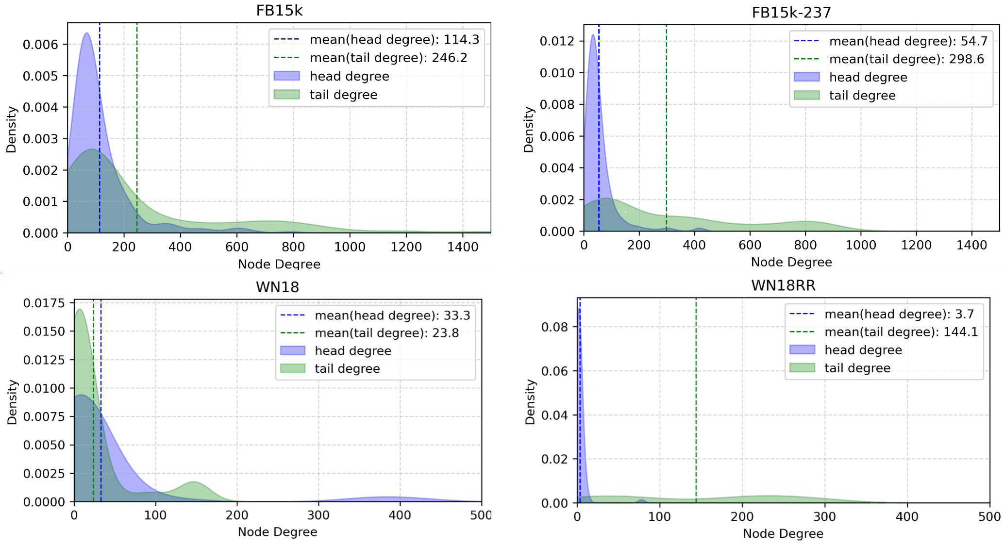
Figure 4: Degree distribution of different datasets and perspectives.

5. As illustrated in Figure 4, we plotted the degree distributions of head and tail entities for $T$ across four datasets. Due to the long-tailed nature of the distributions and the relatively small data size, we plot Kernel Density Estimation (KDE) distributions for each dataset, separately showing the degree distributions of head and tail entities. From the plots, we observe that the degree distributions of head and tail entities in $T$ reflect the characteristics of the datasets. In denser datasets such as FB15k and FB15k-237, tail entities generally exhibit higher degrees than head entities. This observation may also explain why previous eXKGLP methods tend to focus more on triples directly connected to head entities. Additionally, the overall trend of node degrees across datasets follows the order: $FB15k > FB15k-237 > WN18 > WN18RR$.

Review 7: Minor Comments

• Figure 2: What does 81 in the query represent? Should it be 46 instead?
• Figure 4: Missing legend.

Reply: Thank you for pointing this out. We have carefully revised the manuscript to address the errors and improve clarity.

Reviewer 3

Review 1: The benefit of involving the theory on adversarial attacks remains not very clear.

Reply: Thank you for your insightful comment, we have revised Sections 3.2 and 3.3 in the original text to clarify the task background and theoretical foundation of our work. Specifically:

Figure 5: An example of material KG for synthesis route inference. To explain the predicted link ⟨material: BEMHUX, hasSolvent, solvent: DCM⟩ (the dotted red link on the top), classical LP explanations (e.g., Kelpie) will select the single-hop links as explanations (thickened blue links).

The adversarial attack problem (Section 3.2) serves as an empirical evaluation framework for explanations. Specifically, it quantifies the quality of explanations by measuring how minimally modifying the knowledge graph (e.g., removing facts) maximally degrades the prediction score of a target triple. Existing adversarial methods like Kelpie, Criage, and Data Poisoning focus on capturing model-internal signals (e.g., gradient-based sensitivity or embedding shifts) to identify critical facts. While effective, these methods lack semantic justification for why specific facts are deemed critical, reducing their interpretability for human users. For instance, in Fig. 5, they might highlight a fact like $\langle \text{BEMHUX}, \texttt{hasStructure}, \text{CH2Cl2} \rangle$ as critical for predicting $\langle \text{BEMHUX}, \texttt{hasSolvent}, \text{DCM} \rangle$, but fail to explain the underlying causal logic connecting these facts.

To address this gap, we propose path-based adversarial explanations (Section 3.3). Given a prediction $\langle h, r, t\rangle$, our framework identifies the smallest set of training facts whose removal maximally degrades the prediction (adversarial explanation) and provides a path-based rationale justifying why these facts are critical. This rationale is formalized using Closed Path (CP) rules and Property Transition (PT) rules, which generalize relational patterns from the KG into symbolic, human-interpretable structures. For example, CP rules (e.g., $r \leftarrow r_1, r_2$) capture multi-hop dependencies, such as inferring a material's solvent usage through shared substructures (Fig. 5). These rules encode causal semantics, grounding adversarial explanations in domain logic rather than purely computational perturbations (e.g., gradient magnitudes).

The key innovation lies in using ontological rule-based reasoning (CP/PT rules) to enhance adversarial explanations. While adversarial methods efficiently identify critical facts, the rules provide the missing semantic layer, revealing why those facts matter. For instance, in Fig. 5, removing the fact $\langle \text{BEMHUX}, \texttt{hasStructure}, \text{CH2Cl2} \rangle$ degrades the prediction because it disrupts the CP rule connecting sharing substructure: $hasSolvent \leftarrow hasStructure, hasStructure'$. This approach bridges symbolic reasoning (rule semantics) and sub-symbolic adversarial evaluation (score degradation), advancing trust and transparency in domains like healthcare and finance, where explanations must align with human-understandable causality.

To validate our theory, we adopt the adversarial attack framework as an empirical verification tool, similar to KGEAttack's methodology. eXpath mines CP/PT rules from the KG (theory), then evaluates their explanatory power by measuring how removing rule-supported facts degrades predictions, quantified by $\delta$MRR and $\delta$H@1 metrics. Our experiments (Section 5) confirm that rule-anchored explanations achieve 12.4% higher $\delta$MRR than fact-only adversarial methods.

Review 2: Ontology theory (from which closed path rule are borrowed) needs a reference.

Reply: Thank you for raising this point. PT and CP rules defined in this work are inspired by the foundational work of AnyBurl. Specifically, PT rules are derived from AnyBurl's unary rules ending with an atom that includes a constant ($U_c$), with the rule body length restricted to 1. CP rules, on the other hand, are based on AnyBurl's binary rules ($B$). Both types of rules are instances of closed connected rules.

Additionally, the evaluation metrics for CP rules, including support (supp), head coverage (HC), and standard confidence (SC), follow the standard definitions introduced in RLvLR. We have incorporated these references in Section 4.1.

Review 3: Fig 2 (b) is a little bit obscure.

Reply: We appreciate your feedback regarding the clarity of Figure 2(b) in main paper. We acknowledge that the original figure combined multiple steps into a single panel, which made it appear crowded and somewhat obscure. To address this, as shown in Figure 6, we have revised the layout of Figure 2 in main paper to improve its clarity and readability. Specifically, each stage of the pipeline (a, b, c) now contains a single, focused image representing the key step in that stage. For example, stage (b) exclusively illustrates the local optimization process, while stage (c) focuses solely on fact scoring. This separation helps to visually distinguish each step and reduces clutter.

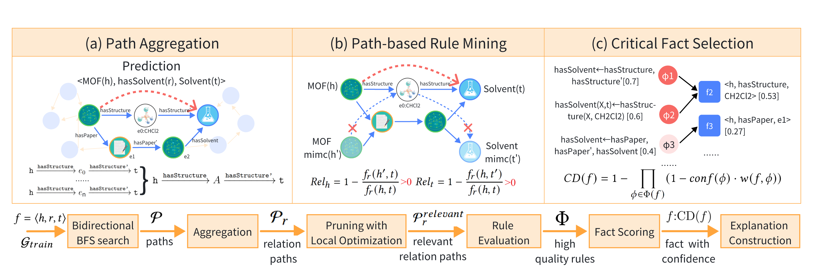
Figure 6: Pipeline of eXpath. (a) Path Aggregation: Identifies paths between $h$ and $t$ using bidirectional BFS and aggregate them into relation paths. (b) Path-based Rule Mining: Prunes relevant relation paths with local optimization and selects high-confidence closed path (CP) and property transition (PT) rules. (c) Critical Fact Selection: Scores candidate facts based on rule weight and confidence, selecting the highest-scoring facts for the final explanation.

To make the figure more concrete, we have used the same case study from Figure 1 to illustrate the entire pipeline. This allows readers to see how the method progresses from identifying paths (stage a) to mining rules (stage b) and finally selecting critical facts (stage c) in a real-world context.

Review 4: End of Section 3 "Thus, directly using multiple paths as explanations will be less effective." What is this related to and how do the authors propose to manage it in the expath method?

Reply: Thank you for your question regarding the statement "Thus, directly using multiple paths as explanations will be less effective." This assertion is tied to the specific task of adversarial attack-based explanations in eXKGLP, where the goal is to identify minimal modifications to the knowledge graph (KG) that have a maximal negative impact on the prediction score. In this context, directly using multiple paths as explanations is not feasible, as it would involve large-scale modifications to the dataset, which deviates from the core objective of the adversarial attack problem. Adversarial attacks require localized, minimal modifications to effectively measure the model's sensitivity to specific facts, and directly using multiple paths would complicate the evaluation of the model's robustness to small perturbations.

Therefore, eXpath does not directly use paths as explanations. Instead, it enhances the existing adversarial explanation by incorporating path-based rationales to provide semantically meaningful justifications for the modifications. Specifically, eXpath identifies a small set of training facts whose removal maximally degrades the prediction score, aligning with the adversarial attack objective of finding impactful, minimal modifications. For selected facts, eXpath provides one or more Closed Path (CP) rules or Property Transition (PT) rules as rationales, which capture semantically meaningful relational patterns in the KG. These rules generalize multi-hop dependencies and attribute transitions, grounding the explanation in causal semantics rather than purely computational perturbations. This hybrid approach ensures that explanations remain computationally efficient while offering deeper interpretability.

Review 5: Section 4.2 resembles typical aspects of association rules mining. What is the difference between this approach and ARM? Is head coverage the same as confidence? This should be discussed briefly.

Reply:
Thank you for your thoughtful feedback. We appreciate the opportunity to clarify these problems.

Traditional ARM methods, such as AMIE, AnyBURL, and RLvLR, focus on mining association rules across the entire KG. These methods are heuristic and aim to discover general rules that apply globally. However, they often suffer from high computational complexity and may not guarantee the completeness of the discovered rules, especially in large-scale KGs. In contrast, our path-based rule mining approach is tailored specifically for embedding-based models and targets only the given prediction. By leveraging mimic-based local optimization, we efficiently prune irrelevant paths and extract high-confidence rules that are directly tied to the model's predictions. This localized focus allows us to achieve efficiency and precision, ensuring that the mined rules are both computationally feasible and semantically meaningful for the specific prediction at hand.

As defined in Equation 4 of the paper, head coverage (HC) and standard confidence (SC) are distinct metrics used to evaluate the quality of rules. In our work, we further refine confidence by introducing a modified version:

$conf(\phi) = SC(\phi) \cdot \frac{supp(\phi)}{supp(\phi) + minSupp}$

where supp denotes the support of the rule. This modification prevents the overestimation of rules with insufficient support (e.g., $supp < 10$), ensuring that only rules with adequate support are generalized.

Review 6: The motivating example in Fig. 1 is different from the example used in Fig. 2. Using the same one would help the understanding.

Reply:
Thank you for your suggestion. We have revised Figure 2 to use the same example as Figure 1, which enhances the consistency and understanding of the pipeline.

Review 7: In Tables 2 and 3 some techniques are combined. I did not find the details on how this has been achieved.

Reply:
We appreciate your feedback. We have added details on how the fusion methods were implemented in Section 5.2. Here is an excerpt from the revised passage:

We evaluate fusion methods (e.g., Kelpie + eXpath) by selecting the explanation that yields the greater reduction in metric between Kelpie and eXpath. Taking $\delta MRR$ as an example, for each fact $f$ to be explained, we define the reciprocal rank of the combined method as $ RR(M_{x+y}, f) = \min(RR(M_x, f), RR(M_y, f)) $. The overall metric for the fusion method is then calculated using the following equation:

$\delta MRR(M_{x+y}, T) = 1 - \frac{\sum_{f\in T} RR(M_{x+y},f)}{\sum_{f\in T} RR(M_o,f)}$

By selecting the minimum value between the two methods, the fusion method enhances explanation performance. The results demonstrate that the path-based explanations of eXpath offer unique insights and complementary perspectives that differ significantly from those provided by other adversarial methods, particularly when combined with Kelpie.

Review 8: The evaluation is very broad but I missed the main message (e.g., in Table 4 I do not see a clear trend) -- it would be better to summarize it at the end and for each part of the section.

Reply:
We appreciate your feedback in strengthening the manuscript's narrative coherence. We have restructured the evaluation section to clarify the main insights and ensure key conclusions are highlighted at the end of each subsection. Below is a summary of the experimental findings:

Section 5.2 (Overall Performance):
Our experiments demonstrate that eXpath generally outperforms existing adversarial explanation methods (Kelpie, DP, KGEAttack) across datasets and models. For single-fact explanations, eXpath achieves an average improvement of 15.4% in $\delta$H@1 and 23.6% in $\delta$MRR compared to baselines. Multi-fact explanations further enhance performance, particularly in dense datasets like FB15k, where four-fact explanations improve $\delta$MRR by 87.7% over single-fact approaches. This highlights the necessity of capturing multi-relational contexts in complex KGs. The fusion of eXpath with non-path methods (e.g., Kelpie) achieves 47% higher $\delta$MRR for single-fact explanations, illustrating the complementary strengths of path-based and fact-centric explanations.

Section 5.3 (Fact Position Preferences):
Table 4 reveals that restricting explanations to head-related facts generally yields the best performance (L1: 0.490 / L4: 0.658), while tail-related facts underperform significantly (L1: 0.413 / L4: 0.501). However, dataset characteristics also influence this trend. In dense KGs like FB15k, unrestricted fact selection (all) outperforms head restrictions, as models balance head and tail entity representations. These findings emphasize the need to adapt fact selection strategies based on graph density: unrestricted selection for dense KGs (average degree >20) and head restrictions for sparse KGs.

Section 5.4 (Ablation Study on Rule Components):
The ablation study (Table 5) confirms that CP rules are the primary driver of eXpath's performance, contributing 13.5%~27% to $\delta$MRR by capturing multi-hop dependencies. PT rules play a complementary role (4.5%~6% contribution), validating co-occurrence patterns. The importance of rules varies by dataset: CP rules dominate in FB15k (relational diversity), while PT rules are critical in FB15k-237 (attribute-rich entities).

Review 9: Why were Criage and Data Poisoning excluded from Table 6?

Reply:
Thank you for your question. Criage and Data Poisoning (DP) were initially excluded from Table 6 because their average performance, as measured by $\delta MRR$ and $\delta H@1$, was weaker compared to KGEAttack and Kelpie. However, we acknowledge that the explanations provided by these methods still hold value for comparative analysis. Therefore, we have updated Table 6 to include columns for Criage and DP, allowing for a side-by-side comparison across three representative cases.

In case (a), both DP and eXpath (L1) generated identical and valid explanations, achieving $\delta MRR=0.89$, while Criage produced an invalid explanation. In case (c), Criage and eXpath (L1) generated the same valid explanation with $\delta MRR=0.33$, whereas DP's explanation was invalid. In case (b), all three methods generated valid explanations, but eXpath achieved higher performance metrics. These results highlight eXpath's robustness and effectiveness in generating meaningful explanations across diverse scenarios.

Review 10: It would be useful to have a description of FB15k, FB15k-237, WN18, and WN18RR (in terms of semantics, in addition to what provided in Table 1), so that also the cases in Table 6 could be understood better.

Reply:
We appreciate your suggestion. In Section 5.1, we have added a description of the FB15k, FB15k-237, WN18, and WN18RR datasets. Here is an excerpt from the revised passage:

As provided in Table 1, FB15k and WN18 are datasets for predicting relationships between entities. FB15k, built from FreeBase (a real-world knowledge base), includes relations like born-in and part-of, but its test data contained reversed relationships, making prediction tasks artificially easy. This led to FB15k-237, a revised version that removes these reversed links. Similarly, WN18, based on WordNet (a semantic network), models linguistic relations like hypernym (e.g., cat is a feline) but suffered from the same flaw. Its improved version, WN18RR, excludes reciprocal relations to ensure fairer evaluation.

Review 11: I do not understand why in Fig 5c all the methods provide considerably different explanations. This should be discussed.

Reply:
Thank you for your feedback. Fig. 5c (corresponding to the case in Table 6(c)) is indeed a coincidental case where the three methods—KGEAttack, Kelpie, and eXpath—generate considerably different explanations. But when Criage and DP are added to the table, we observed that Criage produces the same explanation as eXpath (L1), and DP shares some overlap with Kelpie's explanation. This suggests that despite the apparent differences, there are underlying similarities in the rationale behind these methods' explanations.

Furthermore, the first two examples (a) and (b) demonstrate more overlap among the methods. For instance, in (a), DP, KGEAttack and eXpath share the first fact, and in (b), Kelpie and eXpath share the first two facts. These cases highlight that while the explanations may vary, there are commonalities in the critical facts identified by different methods.